The pruning practice entails targeted removal of diseased, damaged, dead, non-productive, structurally unsound, or otherwise unwanted tissue from crop and landscape plants. [Wikipedia]

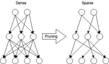
Just as the practice of pruning helps shape and direct the growth of trees and bushes, so does pruning of synaptic connections in the brain play a critical role in learning. The use of pruning in neural network models is gaining popularity due to the many benefits it offers.

Artificial neural networks (ANNs) are traditionally dense and fit the current computing paradigm and architecture of GPUs well. This match between the available hardware and ANN architectures was the major factor that led to the exciting developments in AI within the last decade.

In recent years, novel ANN models have been increasing in size and complexity to such an extent that the memory and computation costs have become a major issue and the focus of the research community [Strubell et al. 2020]. Another consequence is that large models are over-parametrized, which might cause issues with generalization, as the models get too sensitive to subtle input changes [Kohler and Krzyzak 2019, Hoefler et al. 2021]. These issues are usually worked around by using various methods during the training phase, such as:

• L1 or L2 weight regularization
• Dropout regularization variants
• Data Augmentation

However, none of these methods deals with the fundamental issues of over-parametrization: inefficient use of memory and computation.

Pruning or sparsification is a family of methods to produce sparse neural networks. Similar to other regularization methods, pruning often leads to a better generalization of the networks [Bartoldson et al. 2020]. Many recent works have also shown that sparse models tend to be more robust against adversarial attacks [Cosentino et al. 2019; Gopalakrishnanet al.2018; Guo et al.2018; Madaan et al.2020; Rakin et al.2020; Sehwag et al.2020; Verdenius et al.2020]. Sparse models have also significantly lower memory and computation costs compared to dense counterparts (often in the range of 10-100x reduction). This is especially relevant for the training phase because the large and dense models are not only very expensive during inference, but often are prohibitively costly to train [Brown et al. 2020It is important to keep in mind that computation and memory efficiency depend largely on the implementation of the sparse data types and operations on them. Different hardware and different libraries offer a variety of features and support for sparse network models.]. Thus, the pruning methods that are applied during training are the most interesting and beneficial for reducing computational costs.

Typical test error vs. sparsity showing Occam’s hill (results: ResNet-50 on Top-1 ImageNet). Reproduction of Fig. 4 from [Hoefler et al. 2021].

It is important to keep in mind that computation and memory efficiency depend largely on the implementation of the sparse data types and operations on them. Different hardware and different libraries offer a variety of features and support for sparse network models.

Types of sparsity

Different pruning methods can be characterized by three main aspects:

• which parts of the model are pruned
• when is the pruning applied
• how is the pruning implemented

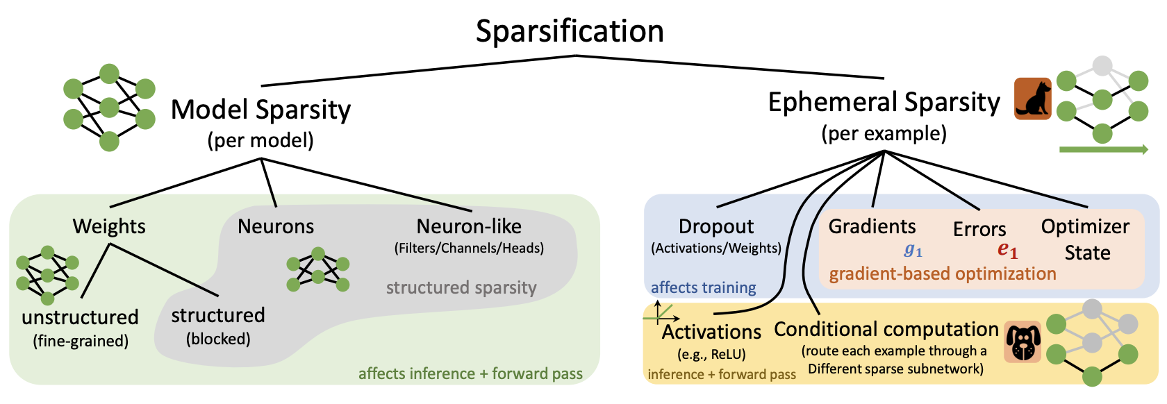
The sparsification or pruning can be permanently applied to the model, also called structural pruning, or temporarily during computation, also called ephemeral sparsification.

Structural pruning in its basic form relates to the fine-grained pruning of weights of a neural network, but can also be applied over larger building blocks of models such as neurons, convolutional filters, and attention heads. Neural architecture search (NAS) is a family of such block pruning methods that aim to automate the search for better deep learning architectures [Elsken et al. 2019]. The advantage of coarser element (block) style pruning is that the block and the architecture of the model stay dense and efficiently executable on common hardware. In contrast, fine-grained pruning of weights can result in unstructured layers which can result in computation and memory overhead depending on the specific architecture and data types used. Fine-grained pruning, however, is much more flexible and when paired with specialized hardware and sparse activations (like neuromorphic chips and spiking neural networks) can result in a much stronger reduction in computation and memory requirements.

Ephemeral sparsification refers to the sparsification happening online, usually dependent on the current input data samples. This type of sparsification is very common in deep learning models and include sparse activations like ReLU, which clamp the output of a neuron to zero for input values below zero, and regularization methods such as Dropout which effectively clamp the output of a random sample of neurons to zero during training. Less common methods that belong to this category include sparsification of gradients during training and conditional computation.

Overview of neural network elements that can be pruned. Reproduction of Fig. 6 from [Hoefler et al. 2021].

When to prune?

Pruning can also be applied at different points during the training of the neural networks. The most trivial and the least beneficial application of pruning is after the training. In this setting, the model is sparsified after the training, which usually results in significant performance degradation. It also means that the full dense model is trained, which is the most costly process in terms of memory and computation.

A better approach is using a schedule of sparsification during training. This way training is started with a dense model which is gradually sparsified during the training procedure. Different pruning schedules and implementation details [Wortsmanet al. 2019; Lin et al. 2020] make this method very flexible. The advantage of this method is that sparsification can prevent overfitting gradually during training. But it can also make convergence more unstable.

[Prechelt 1997] used the generalization loss to quantify the amount of overfitting and adjust the pruning rate dynamically during training. [Jin et al. 2016] combined the dense and sparse training in a single schedule with a method called iterative hard thresholding (IHT). [Han et al. 2017] used a three-step schedule (dense training to convergence, magnitude-pruning followed by retraining, and dense training) and showed that this schedule leads to significantly higher generalization performance. A follow-up extension to this method is presented in [Carreira-Perpinan and Idelbayev 2018]. A major downside to all these approaches is that they still start with dense models which need to be held in memory and thus do not enable the use of smaller-memory devices.

The last category is a fully-sparse training, where training starts with an already sparse model and trains it in the sparse regime by adding and removing weights during training. These methods often have more hyperparameters, but enable very high-dimensional models to be trained on smaller memory hardware. There is a variety of pruning and regrowth techniques that can be combined to implement a fully-sparse training scheme. For example, [Mostafa and Wang 2019] use random regrowth and magnitude pruning to maintain sparsity throughout training.

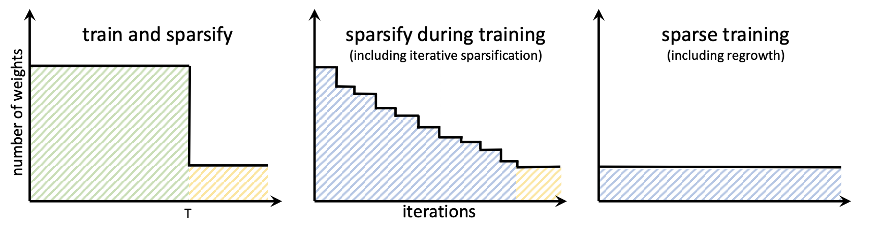
Overview of structural sparsification schedules. Reproduction of Fig. 7 from [Hoefler et al. 2021].

State of the art

Using sparse evolutionary training approach [Mocanu et al., 2018] demonstrates training of sparsely initialized networks by dynamically changing the connectivity with a magnitude-based pruning and random growth strategy. A related method [Bellec et al., 2018] demonstrates the advantage of training sparse networks with stochastic parameter updates, by sampling the sparse connectivity pattern based on a posterior which is theoretically shown to converge to a stationary distribution.

Authors of [Mostafa & Wang, 2019] propose dynamic sparse parameterization to train sparse networks via adaptive threshold-based pruning. In [Dettmers & Zettlemoyer, 2019] authors develop a sparse learning method using momentum-based regrowth of pruned weights.

More recently, with the rising concerns about the adversarial attacks, [Özdenizci and Legenstein 2021] propose an intrinsically sparse rewiring approach based on Bayesian connectivity sampling to train neural networks by simultaneously optimizing the sparse connectivity structure and the robustness-accuracy trade-off.

Summary

In conclusion, the pruning and sparsification of neural networks can provide the following benefits:

• improved generalization
• robustness to adversarial attacks
• memory and compute efficiency

Many popular deep learning libraries already provide many built-in pruning methods:

• TensorFlow
• PyTorch

A large part of the content of this article is based on [Hoefler et al. 2021] and [Özdenizci and Legenstein 2021]. The figures are reproduced with written permission from Prof. Hoefler.