Corrupt, sparse, irregular and ugly: Deep learning on time series
Update 24.06.2020: Thanks to BadInformatics for pointing me to ODE based models and other remarks. The content was extended accordingly.
Update 22.08.2020: Extended the details on missing values; Replaced the first figure with example and code; Added tip for Traces library.
Update 01.11.2021: Added Multi-Time Attention Nets and Neural Rough Differential Equations method
How to train neural networks on time-series that are non-uniformly sampled / irregularly sampled / have non-equidistant timesteps / have missing or corrupt values? In the following post, I try to summarize and point to effective methods for dealing with such data.
What is irregularly sampled data or sequence of non-equidistant steps? 📊
Time series where the time between the individual steps/measurements is not constant is called non-uniform or irregularly sampled. Irregularly sampled data occurs in many fields:
- Meteorological data
- Astronomical data
- Electronic health records (EHRs)
- Turbulence data
- Automotive data
This is also common in cases where the data is multi-modal. Multi-modal input means that the input is coming from multiple different sources which most likely operate and take measurements not synchronized with each other resulting in the non-uniform input data.
Another source of the irregularity in sampling can be missing or corrupt values. This is very common in both automotive and EHR data where sensors malfunction or procedures are interrupted or rescheduled.
Why not just interpolate? 💡
The first idea you might have is to interpolate and resample the time series data at hand. This will produce a uniformly sampled grid and allows for standard methods to be applied. However, this approach works under the strong assumption that the interpolated data behaves monotonically between the measurements. This assumption often does not hold which leads to undesired artifacts during feature transformation and in turn to a sub-par performance (sometimes worse than training on the raw data).
💡 If you are looking for help in transforming unevenly-spaced times series to evenly-spaced ones, check out the Traces python library.
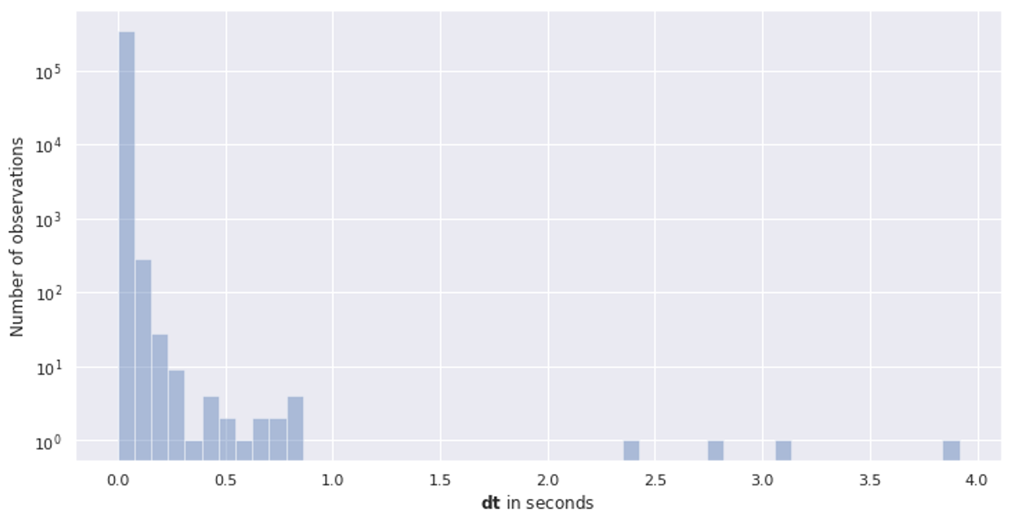
Another factor to consider before interpolating is the distribution of the sizes of timesteps. The easiest way to do this is to plot the histogram of dt-s (time differences) between data points. If the values of dt are relatively large, it is unlikely that the measurements in between the points behave monotonically. Furthermore, you should check the variance of dt and decide whether it is “sufficiently” uniform to apply the classical methods or not, as sometimes it turns out that the data is “uniform enough” (see the next section).
An example of dt distribution of a real world dataset (Gaia European space mission Data Release 2) with irregular time series is shown in the plot below. The plot is generated using this python notebook.
Another factor to consider is the computational and memory cost of interpolation which depends on both the size of your dataset (if you plan to do it offline) and the targeting granularity of the interpolation grid.
However, if you have a sufficiently large amount of data where you could learn the underlying distributions, then it might be worth looking into the methods for data recovery and super-resolution which I describe in the section below.
Solving the problem by ignoring the problem 🙈
There are cases when the variance in the dt-s is small enough and the methods for regularly sampled data can produce surprisingly good results. I would highly suggest first creating a baseline with one such method. For example, you can use any STFT based spectrogram (like MFCC) or any other appropriate spectrogram and train the model using such input.
Having a strong baseline is critical for evaluation of the more advanced input processing methods and the decision if they make sense for your specific setup.
What are the methods for working with irregular or sparse time series? ⚗️
If the distribution of dt is wide in your dataset, then there are several methods for directly dealing with irregularly/nonuniformly sampled data that are worth looking into:
- Lomb-Scargle Periodogram
- Data modeling with Interpolation networks
- Neural Ordinary Differential Equation models ✨
- Add timing dt to the input as an additional feature (or positional encoding)
- Methods for dealing with missing values
How to use Lomb-Scargle Periodograms?
tl;dr Here is a python notebook that shows how to compute a spectrogram of irregularly sampled data using Lomb-Scargle method.
If one wants an actual spectral analysis of non-uniformly sampled signals, then Lomb-Scargle periodogram is a classical method solving the problem. The method is similar to the Fourier Power Spectral Density (PSD), the most popular method for periodicity detection in uniformly/regularly sampled data. Lomb-Scargle Periodogram algorithm has been implemented in many libraries (scipy, gatsby, astropy, matlab), out of which the scipy version should be the most maintained one.
The Lomb-Scargle periodogram was developed by Lomb [Lomb, N.R., 1976] and further extended by Scargle [Scargle, J.D., 1982] to find, and test the significance of weak periodic signals with uneven temporal sampling. [scipy docs]
A periodogram is an estimate of the spectral density of a signal. These libraries provide a method to compute a periodogram (spectral analysis) on a sequence of irregularly sampled values. However, for deep learning we usually need the spectrogram and not a single periodogram.
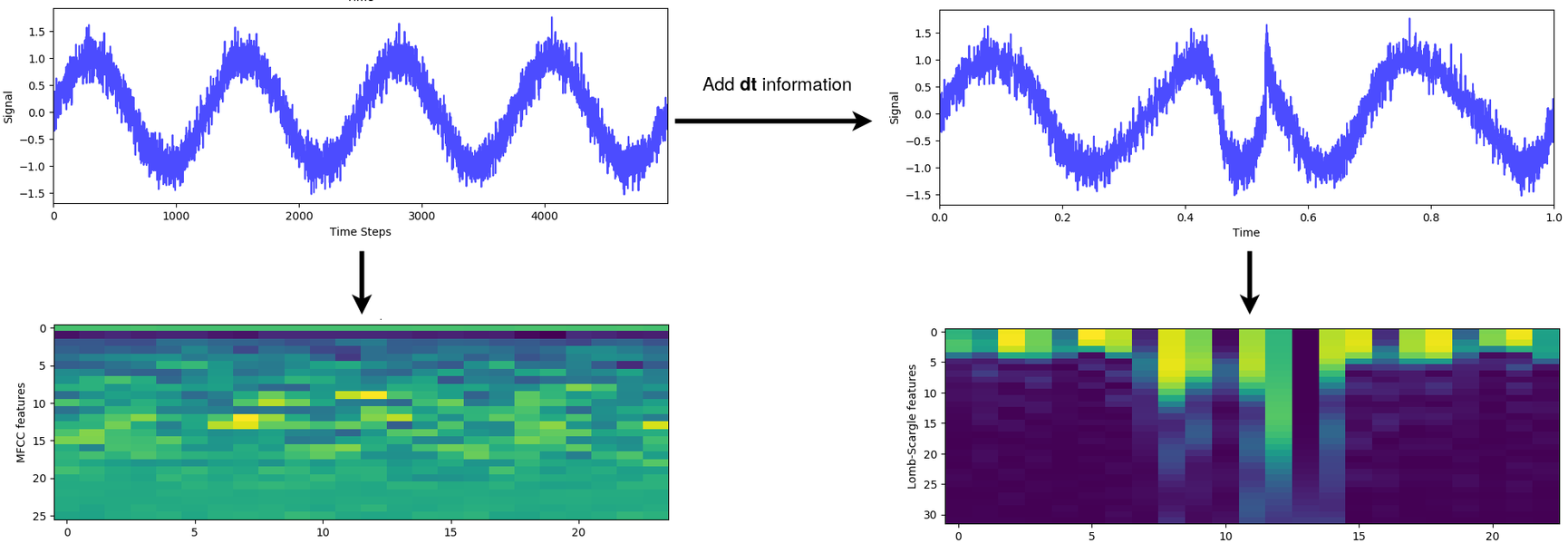
A spectrogram is a representation of the spectral density of frequencies of a signal over time. Thus, we can produce a spectrogram by computing the periodogram over time bins of a signal or time series. Example code on how to do this and that reproduces the figures below, can be found here.
The figure below demonstrates the potential loss of information if we ignore the timing information about the irregular sampling of the data. The figure compares the Short-time Fourier Transform (STFT) based spectrogram (MFCC), which assumes regular sampling, with Lomb-Scargle based spectrogram, which takes dt as additional input. In the top row, we see the signal plot over time-steps (left) and over time (right). This exaggerated synthetic example makes it obvious that the dt can have a significant impact on the signal spectra and thus the spectrogram that does not take the dt into account (bottom left plot) can not detect the true spectral representation of the signal. In the bottom right, the Lomb-Scargle spectrogram is able to capture the change in the signal well.
For further details and more advanced applications of Lomb-Scargle method refer to the following links:
- Lomb-Scargle intuition and important practical considerations
- Extension of Lomb-Scargle to multiband periodogram
- Bayesian formalism for the generalised Lomb-Scargle periodogram
What are interpolation networks?
Researchers dealing with time series data in EHRs are developing data modelling methods that can make use of extremely sparse and irregular data. These models are usually evaluated on classification or regression tasks like predicting the onset or probability of sepsis based on the physiological measurements of a patient.
The common approach involves two stages where the first stage models the trajectories of the irregular and sparse physiological measurements, and the second stage is a common black box prediction neural network.
For example, the first stage in [Shukla and Marlin, 2019] uses a semi-parametric interpolation network [github] to model the data by learning three distinct features: a smooth interpolation for slow trends in the signal, a short time-scale interpolation for transients, and an intensity function for local observation frequencies. An earlier work [Futoma et al., 2017] implements the first stage with multi-task Gaussian processes.
These models attempt to recover the missing information from time-series but only in latent space as the models are trained end-to-end with the prediction neural network on top. However, if your time-series have missing data points, approaches outlined in the section below should be more applicable.
For the scenarios where you have different input channels operating at different frequencies (multi-rate multivariate time series) you should look into [Che et al., 2018b] where the authors deal with this problem using the Multi-Rate Hierarchical Deep Markov Model (MR-HDMM).
For working with physiological signals, it is common to use some form of CNN and/or RNN based architecture [Faust et al., 2018, Fawaz et al., 2019] like 1-D ResNet or architectures based on WaveNet sometimes combined with LSTM or other RNNs.
For efficiently training on sparse, irregularly sampled, and multivariate data the new model called Multi-Time Attention Networks by [Shukla and Marlin 2021] offers great results beating the SOTA benchmarks.
What are Neural Ordinary Differential Equation models?
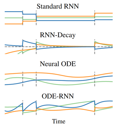
ODE-RNNs [Rubanova et al., 2019] are a novel model that builds upon the original idea of NeuralODEs [Chen et al., 2018] by generalizing the RNNs to have continuous-time hidden dynamics. In short, they are a natural fit to solve irregularly sampled time series data problems and outperform the RNN counterparts in that domain. This is best summarized in this excerpt from the paper abstract:
“Both ODE-RNNs and Latent ODEs can naturally handle arbitrary time gaps between observations, and can explicitly model the probability of observation times using Poisson processes. We show experimentally that these ODE-based models outperform their RNN-based counterparts on irregularly-sampled data.” [Rubanova et al., 2019]
A downside of the ODE based models is that the solution to an ordinary differential equation is determined by its initial condition. The follow-up work [Kidger et al., 2020] deals with this issue using the controlled differential equations and set the new state-of-the-art. The newly introduced Neural CDE outperforms ODE-RNNs and GRU-D models on CharacterTrajectories, PhysioNet, and Speech Commands dataset.
How to make an input feature out of timestamps? ⏱️
Usually, timseries data contains a timestamp for each data point. The first thing to do is to convert the timestamps to delta t-s (dts). Next, you will need to perform a cumulative sum on the dt feature to get a monotonically increasing value. Finally, you might need to standardize the values (scale to the range [0, 1]) if your model always works with uniformly long sequences at the input.
Depending on the problem, if your model is sometimes working on a subsequence of a much longer input stream and needs to be aware of the position in the stream, then computing a cumulative sum of dts beforehand might be required and the standardization needs to be omitted. Otherwise, the model would not receive the contextual information (position in the input stream) which could potentially have a significant impact on the performance of the model.
Finally, the newly computed feature can be provided to the models as additional input.
This method can also be seen as a form of positional encoding of the Transformer to deal with irregularly sampled data. The added dt based feature allows the attention layer to compute the similarity (distance) between the data points using the precise timing information in addition to the other features.
How to deal with missing values in time-series? 🔍
To effectively model the data with missing values it is important to understand the cause of the missing data. For example, if the data is missing at random, the rest of the data is still representative and well suited for modelling. However, if the missing values do not occur at random, the rest of the data will be biased. In statistics, different types of missing data are classified as:
- Missing completely at random (MCAR)
- Missing at random (MAR)
- Missing not at random (MNAR)
To minimize the work required to analyze, identify and deal with these different types of missing values, deep learning methods have been developed that can deal with these issues directly. Such models take the information about the missing values along with the available data and are trained end-to-end for a specific task, resulting in more accurate models that are aware of the statistics of the missing values.
For dealing with missing values in multivariate time series the authors of [Che et al., 2018a] propose the GRU-D model which ingests the explicit representation of missing values (masking and time interval) and incorporates them into the architecture. This way the model can exploit not only the long-term temporal dependencies but also the patterns of missing values.
Beware that ODE-RNNs [Rubanova et al., 2019] outperform GRU-D on some benchmarks.
If you have a vast amount of data, it might also be fruitful to look into the methods for the reconstruction of irregularly and regularly missing data [[Chai et al.]](https://www.nature.com/articles/s41598-020-59801-x#Bib1). This is an analogous approach to the image and audio super-resolution networks. Using this approach you can learn the underlying distribution of your data which is usually a crucial factor in getting a high performing model.
Further reading 📚
If you wish for more references to papers dealing with this topic, I would highly recommend the related work section of [Rubanova et al., 2019].
For a review on interpretability of models for sequential data see [Shickel and Rashidi, 2020].
For dealing with very long time series check out [Morrill et al. 2021] along with the code where the authors apply a unique ODE method to efficiently train RNNs on unfeasibly long time series.
Final note 🎵
To choose the right approach for your specific case it is very important to analyze and understand your own data before getting lost in the rabbit hole of experimentation with all the different approaches that potentially might work. This is only one of the point from the best practice guidelines for deep learning which you should religiously follow if you value your time.
Hope this was helpful and you were able to get some useful pointers and links that will help with your deep learning endeavors. Cheers! 🍻